Binary Threshold Level Selection
Binary Threshold Level Selection - Java Tutorial
When creating a binary image having only two intensity levels (black and white) from an original grayscale digital image that has 256 possible intensity values (for an 8-bit image), a binary threshold level must be chosen to designate the intensity level at which binary segregation occurs. This interactive tutorial explores the use of various algorithms utilized in the methodology for choosing a single binary threshold level. The more general case of multiple threshold level selection is discussed in the Binary Slicing tutorial.
The tutorial initializes with a randomly selected specimen image (captured in the microscope) appearing in the left-hand window entitled Specimen Image. Each specimen name includes, in parentheses, an abbreviation designating the contrast mechanism employed in obtaining the image. The following nomenclature is used: (FL), fluorescence; (BF), brightfield; (DF), darkfield; (PC), phase contrast; (DIC), differential interference contrast (Nomarski); (HMC), Hoffman modulation contrast; and (POL), polarized light. Visitors will note that specimens captured using the various techniques available in optical microscopy behave differently during image processing in the tutorial.
Adjacent to the Specimen Image window is the Grayscale Histogram window that displays the gray-level histogram derived from the original specimen image. To operate the tutorial, select a specimen image using the Choose A Specimen pull-down menu. After examining the original grayscale image, select the binary form of the specimen image for viewing by clicking on the Binary radio button in the Display Image radio button collection. The two images can be compared by toggling between the Binary and Original Grayscale radio button selections. Visitors are encouraged to explore the effects of applying the various threshold-level selection algorithms available in the Choose A Method pull-down menu to the images available in the Specimen Image menu.
Binary images have a limited pixel intensity range consisting of only two possible values: on or off (or one and zero, respectively). In the tutorial, a pixel that is on is represented by the maximum gray-level intensity of white (one), and a pixel that is off is represented by the minimum gray-level intensity of black (zero).
Binary segmentation involves setting a pixel on or off depending on how it compares to a pre-selected threshold level. In the tutorial, a pixel in the specimen image is turned off if its gray-level intensity is less than the threshold level, and a pixel is turned on if its gray-level intensity is greater than or equal to the threshold level. The binary threshold level is indicated in the Grayscale Histogram window by a red vertical line.
Binary segmentation is intended to reduce the vast information content of a grayscale image, while at the same time ensuring that the features of interest remain recognizable. The technique is often used in optical microscopy for analysis of specimen features, because a large number of feature recognition and classification algorithms operate exclusively on binary images.
The choice of a threshold level can have a significant impact on the appearance of the resulting binary image. When choosing a threshold level, it is desirable to include the features of interest among the on (or white) pixels, while reserving the background pixels that lack specimen information among the off (or black) pixels. For an 8-bit gray-level digital image, there are a total of 256 possible choices for binary threshold level. In the tutorial, it is possible to set the threshold level on the specimen image to any of the 256 gray-levels by selecting the Level Selection option from the Choose A Method pull-down menu and using the accompanying Threshold Level slider that appears beneath the histogram. Although interactive selection of an appropriate threshold level may be adequate for a single or small handful of images, automatic selection methods are preferable for processing large quantities of digital images.
When a large number of similar specimen images are captured under identical conditions, then it is often feasible to choose a single threshold level based on a subset of the images and then to apply this threshold level to all of the images in the collection. A similar approach involves segmenting a group of images according to a fixed ratio of black pixels to white pixels, with the ratio being selected appropriate to the particular image set. In the tutorial, the Percent Black Selection method (selectable from the Choose A Method pull-down menu) enables the user to specify a percentage of black pixels desired in the binary image with the Percent Black Pixels slider. A simple algorithm for determining the threshold level for a given image (and the percentage of black pixels desired) operates by computing the smallest nonnegative integer K such that the following relation is satisfied:

In the equation above, N represents the total number of pixels in the image, p represents the percentage of black pixels desired, and h represents the image histogram sequence. This method is automatic in the sense that the threshold gray-level for a particular image will be calculated algorithmically, but it is not automatic in the sense that the user must choose the percentage of black pixels desired.
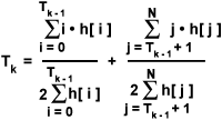
One truly automatic algorithm for choosing a binary threshold level is known as iterative selection. This technique employs an algorithm that sequentially refines an initial estimate of a suitable threshold level. After the threshold level has been estimated, iterative selection operates by segregating the image pixels into specimen and background classes. The algorithm then utilizes the gray levels contained in each class to improve the initial threshold level estimate, which is the mean gray level of the image. On each iteration, the mean gray level for all pixels below the threshold is determined, and is denoted as T(B). The mean gray level for all pixels greater than or equal to the threshold level is also determined, and is denoted as T(W). The new estimate is computed as the arithmetic mean or average of T(B) and T(W), or (T(B) + T(W)) / 2. A general equation for computing the kth estimate of the threshold using the image histogram h is:

In this equation, T(0) represents the initial estimate of the threshold level. The algorithm terminates when T(B) and T(W) are equal, or when T(k) = T(k - 1). In the tutorial, the Mean Iterative Selection method (selectable from the Choose A Method pull-down menu) illustrates the effects of applying this algorithm to find a binary threshold level.
Another method of automatic threshold selection is based on viewing the gray-level histogram of an image as an estimated probability density function of the gray-levels comprising specimen and background pixels. If the specimen pixels and background pixels in the image are each considered to be normally distributed but contained in separate classes, then the gray-level histogram can be seen as an approximation to the sum of two normal distributions given by the equation:

In the equation above, μ(k) and σ(k) (for k = 1, 2) represent the mean and variance, respectively, of gaussian distributions that approximate the specimen and background pixel distributions. Minimum error binary segmentation is an algorithm that operates by arbitrarily dividing the histogram into two parts, modeling each part with a normal distribution, and comparing the combined models with the original histogram. The threshold level that minimizes the discrepancy between the model and the histogram is the one that displays a minimum error. The operation of this algorithm is illustrated in the tutorial with the Minimum Error method (selectable from the Choose A Method pull-down menu).
Other methods of automatic binary segmentation rely on the concept of entropy, a term describing a measure of information content. In this sense, entropy represents a quantitative description of the amount of information in a message based on the logarithm of the number of the possible equivalent messages. If the information content of an image can be represented with N possible values (or gray-levels), and the value x will occur with probability p(x), then the entropy of the image is given by:

Entropy is typically measured in bits per symbol (gray level). In terms of grayscale digital images, the greater the entropy of the image gray levels, the higher the number of bits required in order to create an adequate representation of the information content. A grayscale image having high information content in this sense will also have a broad dynamic range. If the black and white pixels are considered as separate classes with distinct symbol sets, then a measure of entropy can be separately defined for each class. Thus, one approach to choosing a suitable threshold level is to attempt to maximize the entropy of the black and white pixel classes simultaneously. This approach attempts to ensure that the combined entropy of the black and white pixel classes is optimized in an effort to avoid selecting a threshold level that renders the resulting binary image nearly all black or all white. The technique also assumes that the object and background pixel classes in the original grayscale image each have adequate entropy. An implementation of an entropy-based algorithm is available in the tutorial with the Entropy Selection method (selectable from the Choose A Method pull-down menu).
The idea of fuzzy sets has also been employed in the design of automatic binary thresholding algorithms. In fuzzy set theory, given a set S, an element x belongs to S with a probability P(x). When applying this idea to the problem of binary segmentation, a pixel in the grayscale image can be assigned a probability of belonging to either the set of specimen pixels or the set of background pixels. A measure based on the idea of fuzziness can be defined that quantifies the difference between the original grayscale image and the binary image. Determining the threshold level that minimizes the fuzziness measure will produce a binary image having the most accurate rendition of the original grayscale image.
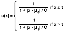
The first step of this process is to define the membership function, or the probability associated with each pixel belonging to the set of specimen pixels or the set of background pixels. One possible condition for the membership function is that, the smaller the difference between the gray level of any pixel x and the mean for its class, the greater will be the value of the membership function u(x). A membership function that fulfills this condition is:

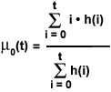
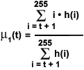
In the equation above, t signifies a given threshold gray level, C is a constant that represents the difference between the maximum and minimum gray levels present in the grayscale image, µ(0) is the mean value of the background pixel class, and µ(1) is the mean value of the specimen pixel class. The upper equation of the membership function applies to background pixels, and the lower equation applies to specimen pixels. In either case, the membership function assigns a numerical probability between 0.5 and 1 to the degree that a pixel belongs in one of the two classes. The means of the background and specimen pixel classes, µ(0) and µ(1), are defined for a given threshold level t as follows:


The next step is to determine a measure of the fuzziness of the segmentation for a given threshold level t. One method for measuring fuzziness is based on the idea of the entropy of a fuzzy set, which is calculated using Shannon's function, or:
Hf(x) = -x log(x) - (1 - x) log(1 - x)
The entropy of the entire image is then given by:

In the equation above, the summation is taken over all of the possible gray levels, and N is the total number of pixels in the image. The algorithm operates by finding the threshold gray level that minimizes the entropy of the fuzziness measure. The results of applying this algorithm are illustrated in the tutorial by the Fuzzy Minimum Error option that is selectable from the Choose A Method pull-down menu.
Currently, many methods of automatic binary segmentation are widely utilized in various applications of computer vision. Other automatic binary segmentation techniques that are not examined in this tutorial include regional threshold selection algorithms, which are often successful in compensating for uneven illumination. A number of other methods of automatic threshold selection have been devised using statistical notions, entropy, and edge detection. Because binary segmentation is often a necessary first step in performing operations such as skeletonization, dilation and erosion, as well as feature identification, measurement, and counting, automatic threshold level selection presents itself as a potentially useful technique for a wide range of applications in microscopy.
Sorry, this page is not
available in your country.